Release 8.0
A58246-01
Library |
Product |
Contents |
Index |
| Oracle8 Tuning Release 8.0 A58246-01 |
|
![]()
![]()
Parallel execution can dramatically reduce response time for data-intensive operations on very large databases. This chapter explains how to tune your system for optimal performance of parallel operations.
See Also: Oracle8 Concepts, for basic principles of parallel execution.
See your operating system-specific Oracle documentation for more information about tuning while using parallel execution.
Parallel execution is useful for operations that access a large amount of data by way of large table scans, large joins, the creation of large indexes, partitioned index scans; bulk inserts, updates, deletes; aggregation or copying. It benefits systems with all of the following characteristics:
If any one of these conditions is not true for your system, parallel execution may not significantly help performance. In fact, on over-utilized systems or systems with small I/O bandwidth, parallel execution can impede system performance.
Note: In this chapter the term "parallel server process" designates a process (or a thread, on NT systems) that is performing a parallel operation, as distinguished from the product "Oracle Parallel Server".
Many initialization parameters affect parallel execution performance. For best results, start with an initialization file that is appropriate for the intended application.
Before starting the Oracle Server, set the initialization parameters described in this section. The recommended settings are guidelines for a large data warehouse (more than 100 gigabytes) on a typical high-end shared memory multiprocessor with one or two gigabytes of memory. Each section explains how to modify these settings for other configurations. Note that you can change some of these parameters dynamically with ALTER SYSTEM or ALTER SESSION statements. The parameters are grouped as follows:
The parameters discussed in this section affect the consumption of memory and other resources for all parallel operations, and in particular for parallel query. Chapter 20, "Understanding Parallel Execution Performance Issues" describes in detail how these parameters interrelate.
You must configure memory at two levels:
The SGA is typically part of the real physical memory. The SGA is static, of fixed size; if you want to change its size you must shut down the database, make the change, and restart the database.
The memory used in data warehousing operations is much more dynamic. It comes out of process memory: and both the size of a process' memory and the number of processes can vary greatly.
Process memory, in turn, comes from virtual memory. Total virtual memory should be somewhat larger than available real memory, which is the physical memory minus the size of the SGA. Virtual memory generally should not exceed twice the size of the physical memory less the SGA size. If you make it many times more than real memory, the paging rate may go up when the machine is overloaded at peak times.
As a general guideline for memory sizing, note that each process needs address space big enough for its hash joins. A dominant factor in heavyweight data warehousing operations is the relationship between memory, number of processes, and number of hash join operations. Hash joins and large sorts are memory-intensive operations, so you may want to configure fewer processes, each with a greater limit on the amount of memory it can use. Bear in mind, however, that sort performance degrades with increased memory use.
Recommended value: Hash area size should be approximately half of the square root of S, where S is the size (in MB) of the smaller of the inputs to the join operation. (The value should not be less than 1MB.)
This relationship can be expressed as follows:![]()
For example, if S equals 16MB, a minimum appropriate value for the hash area might be 2MB, summed over all the parallel processes. Thus if you have 2 parallel processes, a minimum appropriate size might be 1MB hash area size. A smaller hash area would not be advisable.
For a large data warehouse, HASH_AREA_SIZE may range from 8MB to 32MB or more.
This parameter provides for adequate memory for hash joins. Each process that performs a parallel hash join uses an amount of memory equal to HASH_AREA_SIZE.
Hash join performance is more sensitive to HASH_AREA_SIZE than sort performance is to SORT_AREA_SIZE. As with SORT_AREA_SIZE, too large a hash area may cause the system to run out of memory.
The hash area does not cache blocks in the buffer cache; even low values of HASH_AREA_SIZE will not cause this to occur. Too small a setting could, however, affect performance.
Note that HASH_AREA_SIZE is relevant to parallel query operations, and to the query portion of DML or DDL statements.
See Also: "SORT_AREA_SIZE" on page 19-12
Recommended value: 100/number_of_concurrent_users
This parameter determines how aggressively the optimizer attempts to parallelize a given execution plan. OPTIMIZER_PERCENT_PARALLEL encourages the optimizer to use plans that have low response time because of parallel execution, even if total resource used is not minimized.
The default value of OPTIMIZER_PERCENT_PARALLEL is 0, which parallelizes the plan that uses the least resource, if possible. Here, the execution time of the operation may be long because only a small amount of resource is used. A value of 100 causes the optimizer always to choose a parallel plan unless a serial plan would complete faster.
Note: Given an appropriate index a single record can be selected very quickly from a table, and does not require parallelism. A full scan to find the single row can be executed in parallel. Normally, however, each parallel process examines many rows. In this case response time of a parallel plan will be higher and total system resource use will be much greater than if it were done by a serial plan using an index. With a parallel plan, the delay is shortened because more resource is used. The parallel plan could use up to D times more resource, where D is the degree of parallelism. A value between 0 and 100 sets an intermediate trade-off between throughput and response time. Low values favor indexes; high values favor table scans.
A nonzero setting of OPTIMIZER_PERCENT_PARALLEL will be overridden if you use a FIRST_ROWS hint or set OPTIMIZER_MODE to FIRST_ROWS.
Recommended value: 2 * CPUs * number_of_concurrent_users
Most parallel operations need at most twice the number of parallel server processes (sometimes called "query servers") as the maximum degree of parallelism attributed to any table in the operation. By default this is at most twice the number of CPUs. The following figure illustrates how the recommended value is derived.
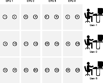
To support concurrent users, add more parallel server processes. You probably want to limit the number of CPU-bound processes to be a small multiple of the number of CPUs (perhaps 4 to 16 times the number of CPUs). This would limit the number of concurrent parallel execution statements to be in the range of 2 to 8.
Note that if a database's users start up too many concurrent operations, Oracle may run out of parallel server processes. In this case, Oracle executes the operation sequentially or gives an error if PARALLEL_MIN_PERCENT is set.
When concurrent users use too many parallel server processes, memory contention (paging), I/O contention, or excessive context switching can occur. This contention could reduce system throughput to a level lower than if no parallel execution were used. Increase the PARALLEL_MAX_SERVERS value only if your system has sufficient memory and I/O bandwidth for the resulting load. Limiting the total number of parallel server processes may restrict the number of concurrent users that can execute parallel operations, but system throughput will tend to remain stable.
To increase the number of concurrent users, you could restrict the number of concurrent sessions that various classes of user can have. For example:
You can limit the amount of parallelism available to a given user by setting up a resource profile associated with the user. In this way you can limit the number of sessions or concurrent logons, which limits the number of parallel processes the user can have. (Each parallel server process working on your parallel execution statement is logged on as you-it counts against your limit of concurrent sessions.) For example, to limit a user to 10 processes, the DBA would set the user's limit to 11: one process for the parallel coordinator, and ten more parallel processes which would consist of two server sets. The user's maximum degree of parallelism would thus be 5.
On Oracle Parallel Server, if you have reached the limit of PARALLEL_MAX_SERVERS on an instance and you attempt to query a GV$ view, one additional parallel server process will be spawned for this purpose. The extra process is not available for any parallel operation other than GV$ queries.
Recommended value: PARALLEL_MAX_SERVERS
The system parameter PARALLEL_MIN_SERVERS allows you to specify the number of processes to be started and reserved for parallel operations at startup in a single instance. The syntax is:
PARALLEL_MIN_SERVERS=n
where n is the number of processes you want to start and reserve for parallel operations. Sometimes you may not be able to increase the maximum number of parallel server processes for an instance, because the maximum number depends on the capacity of the CPUs and the I/O bandwidth (platform-specific issues). However, if servers are continuously starting and shutting down, you should consider increasing the value of the parameter PARALLEL_MIN_SERVERS.
For example, if you have determined that the maximum number of concurrent parallel server processes that your machine can manage is 100, you should set PARALLEL_MAX_SERVERS to 100. Next determine how many parallel server processes the average operation needs, and how many operations are likely to be executed concurrently. For this example, assume you will have two concurrent operations with 20 as the average degree of parallelism. At any given time, there could be 80 parallel server processes busy on an instance. You should therefore set the parameter PARALLEL_MIN_SERVERS to 80.
Consider decreasing PARALLEL_MIN_SERVERS if fewer parallel server processes than this value are typically busy at any given time. Idle parallel server processes constitute unnecessary system overhead.
Consider increasing PARALLEL_MIN_SERVERS if more parallel server processes than this value are typically active, and the "Servers Started" statistic of V$PQ_SYSSTAT is continuously growing.
The advantage of starting these processes at startup is the reduction of process creation overhead. Note that Oracle reserves memory from the shared pool for these processes; you should therefore add additional memory using the initialization parameter SHARED_POOL_SIZE to compensate. Use the following formula to determine how much memory to add:
(CPUs + 2) * (PARALLEL_MIN_SERVERS) * 1.5 * (BLOCK_SIZE)
Recommended value: FALSE
On sites that have no clear usage profile, no consistent pattern of usage, you can use the PARALLEL_ADAPTIVE_MULTI_USER parameter to tune parallel execution for a multi-user environment. When set to TRUE, this parameter automatically reduces the requested degree of parallelism based on the current number of active parallel execution users on the system. The effective degree of parallelism is based on the degree of parallelism set by the table attributes or hint, divided by the total number of parallel execution users. Oracle assumes that the degree of parallelism provided has been tuned for optimal performance in a single user environment.
Note: This approach may not be suited for the general tuning policies you have implemented at your site. For this reason you should test and understand its effects, given your normal workload, before deciding to use it.
Note in particular that the degree of parallelism is not dynamic, but adaptive. It works best during a steady state when the number of users remains fairly constant. When the number of users increases or decreases drastically, the machine may be over- or under-utilized. For best results, use a parallel degree which is slightly greater than the number of processors. Based on available memory, the system can absorb an extra load. Once the degree of parallelism is chosen, it is kept during the entire query.
Consider, for example, a 16 CPU machine with the default degree of parallelism set to 32. If one user issues a parallel query, that user gets a degree of 32, effectively utilizing all of the CPU and memory resources in the system. If two users issue parallel queries, each gets a degree of 16. As the number of users on the system increases, the degree of parallelism continues to be reduced until a maximum of 32 users are running with degree 1 parallelism.
This parameter works best when used in single-node symmetric multiprocessors (SMPs). However, it can be set to TRUE when using Oracle Parallel Server if all of the following conditions are true:
* All parallel execution users connect to the same node.
* Instance groups are not configured.
* Each node has more than one CPU.
In this case, Oracle attempts to reduce the instances first, then the degree. If any of the above conditions is not met, and the parameter is set to TRUE, the algorithm may reduce parallelism excessively, causing unnecessary idle time.
Increase the initial value of this parameter to provide space for a pool of message buffers that parallel server processes can use to communicate with each other.
Note: The message buffer size might be 2 K or 4 K, depending on the platform. Check your platform vendor's documentation for details.
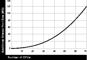
As illustrated in the following figure, assuming 4 concurrent users and 2 K buffer size, you would increase SHARED_POOL_SIZE by 6 K * (CPUs + 2) * PARALLEL_MAX_SERVERS for a pool of message buffers that parallel server processes use to communicate. This value grows quadratically with the degree of parallelism, if you set PARALLEL_MAX_SERVERS to the recommended value. (This is because the recommended values of PARALLEL_MAX_SERVERS and SHARED_POOL_SIZE both are calculated using the square root of the number of CPUs-a quadratic function.)
Parallel plans take up about twice as much space in the SQL area as serial plans, but additional space allocation is probably not necessary because generally they are not shared.
On Oracle Parallel Server, multiple CPUs can exist in a single node, and parallel operation can be performed across nodes. Whereas symmetric multiprocessor (SMP) systems use 3 buffers for connection, 4 buffers are used to connect between instances on Oracle Parallel Server. Thus you should normally have 4 buffers in shared memory: 2 in the local shared pool and 2 in the remote shared pool. The formula for increasing the value of SHARED_POOL_SIZE on Oracle Parallel Server becomes:
(4 * msgbuffer_size) * ((CPUs_per_node * #nodes ) + 2) * (PARALLEL_MAX_SERVERS * #nodes)
Note that the degree of parallelism on Oracle Parallel Server is expressed by the number of CPUs per node multiplied by the number of nodes.
Sample Range: 256 K to 4 M
This parameter specifies the amount of memory to allocate per parallel server process for sort operations. If memory is abundant on your system, you can benefit from setting SORT_AREA_SIZE to a large value. This can dramatically increase the performance of hash operations, because the entire operation is more likely to be performed in memory. However, if memory is a concern for your system, you may want to limit the amount of memory allocated for sorts and hashing operations. Instead, increase the size of the buffer cache so that data blocks from temporary sort segments can be cached in the buffer cache.
If the sort area is too small, an excessive amount of I/O will be required to merge a large number of runs. If the sort area size is smaller than the amount of data to sort, then the sort will spill to disk, creating sort runs. These must then be merged again using the sort area. If the sort area size is very small, there will be many runs to merge, and multiple passes may be necessary. The amount of I/O increases as the sort area size decreases.
If the sort area is too large, the operating system paging rate will be excessive. The cumulative sort area adds up fast, because each parallel server can allocate this amount of memory for each sort. Monitor the operating system paging rate to see if too much memory is being requested.
Note that SORT_AREA_SIZE is relevant to parallel query operations and to the query portion of DML or DDL statements. All CREATE INDEX statements must do some sorting to generate the index. These include:
See Also: "HASH_AREA_SIZE" on page 19-4
Parallel INSERT, UPDATE, and DELETE require more resources than do serial DML operations. Likewise, PARALLEL CREATE TABLE ... AS SELECT and PARALLEL CREATE INDEX may require more resources. For this reason you may need to increase the value of several additional initialization parameters. Note that these parameters do not affect resources for queries.
See Also: Oracle8 SQL Reference for complete information about parameters.
For parallel DML, each parallel server process starts a transaction. The parallel coordinator uses the two-phase commit protocol to commit transactions; therefore the number of transactions being processed increases by the degree of parallelism. You may thus need to increase the value of the TRANSACTIONS initialization parameter, which specifies the maximum number of concurrent transactions. (The default assumes no parallelism.) For example, if you have degree 20 parallelism you will have 20 more new server transactions (or 40, if you have two server sets) and 1 coordinator transaction; thus you should increase TRANSACTIONS by 21 (or 41), if they are running in the same instance.
The increased number of transactions for parallel DML necessitates many rollback segments. For example, one command with degree 5 parallelism uses 5 server transactions, which should be distributed among different rollback segments. The rollback segments should belong to tablespaces that have free space. The rollback segments should be unlimited, or you should specify a high value for the MAXEXTENTS parameter of the STORAGE clause. In this way they can extend and not run out of space.
Check the statistic "redo buffer allocation retries" in the V$SYSSTAT view. If this value is high, try to increase the LOG_BUFFER size. A common LOG_BUFFER size for a system generating lots of logs is 3 to 5MB. If the number of retries is still high after increasing LOG_BUFFER size, a problem may exist with the disk where the log buffers reside. In that case, stripe the log files across multiple disks in order to increase the I/O bandwidth.
Note that parallel DML generates a good deal more redo than does serial DML, especially during inserts, updates and deletes.
This parameter specifies the maximum number of DML locks. Its value should equal the grand total of locks on tables referenced by all users. A parallel DML operation's lock and enqueue resource requirement is very different from serial DML. Parallel DML holds many more locks, so you should increase the value of the ENQUEUE_RESOURCES and DML_LOCKS parameters, by a equal amounts.
The following table shows the types of lock acquired by coordinator and server processes, for different types of parallel DML statements. Using this information you can figure the value required for these parameters. Note that a server process can work on one or more partitions, but a partition can only be worked on by one server process (this is different from parallel query).
Note: Table, partition, and partition-wait DML locks all appear as TM locks in the V$LOCK view.
Consider a table with 600 partitions, running with parallel degree 100, assuming all partitions are involved in the parallel UPDATE/DELETE statement.
|
The coordinator acquires: |
1 table lock SX |
|
|
600 partition locks X |
|
Total server processes acquire: |
100 table locks SX |
|
|
600 partition locks NULL |
|
|
600 partition-wait locks X |
This parameter sets the number of resources that can be locked by the distributed lock manager. Parallel DML operations require many more resources than serial DML. Therefore, you should increase the value of the ENQUEUE_RESOURCES and DML_LOCKS parameters, by equal amounts.
See Also: "DML_LOCKS" on page 19-14
Set these parameters in order to use the latest available Oracle 8 functionality.
Note: Use partitioned tables instead of partition views. Partition views will be obsoleted in a future release.
Recommended value: HASH
When set to HASH, this parameter causes the NOT IN operator to be evaluated in parallel using a parallel hash anti-join. Without this parameter set to HASH, NOT IN is evaluated as a (sequential) correlated subquery.
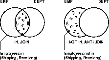
As illustrated above, the SQL IN predicate can be evaluated using a join to intersect two sets. Thus emp.deptno can be joined to dept.deptno to yield a list of employees in a set of departments.
Alternatively, the SQL NOT IN predicate can be evaluated using an anti-join to subtract two sets. Thus emp.deptno can be anti-joined to dept.deptno to select all employees who are not in a set of departments. Thus you can get a list of all employees who are not in the Shipping or Receiving departments.
For a specific query, place the MERGE_AJ or HASH_AJ hints into the NOT IN subquery. MERGE_AJ uses a sort-merge anti-join and HASH_AJ uses a hash anti-join.
For example:
SELECT * FROM emp
WHERE ename LIKE 'J%' AND
deptno IS NOT NULL AND
deptno NOT IN (SELECT /*+ HASH_AJ */ deptno FROM dept
WHERE deptno IS NOT NULL AND
loc = 'DALLAS');
If you wish the anti-join transformation always to occur if the conditions in the previous section are met, set the ALWAYS_ANTI_JOIN initialization parameter to MERGE or HASH. The transformation to the corresponding anti-join type then takes place whenever possible.
Recommended value: default
When set to HASH, this parameter converts a correlated EXISTS subquery into a view query block and semi-join which is evaluated in parallel.
For a specific query, place the HASH_SJ or MERGE_SJ hint into the EXISTS subquery. HASH_SJ uses a hash semi-join and MERGE_SJ uses a sort merge semi-join. For example:
SELECT * FROM t1 WHERE EXISTS (SELECT /*+ HASH_SJ */ * FROM t2WHERE t1.c1 = t2.c1 AND t2.c3 > 5);
This converts the subquery into a special type of join between t1 and t2 that preserves the semantics of the subquery; that is, even if there is more than one matching row in t2 for a row in t1, the row in t1 will be returned only once.
A subquery will be evaluated as a semi-join only with the following limitations:
If you wish the semi-join transformation always to occur if the conditions in the previous section are met, set the ALWAYS_SEMI_JOIN initialization parameter to HASH or MERGE. The transformation to the corresponding semi-join type then takes place whenever possible.
Sample Value: 8.0.0
This parameter enables new features that may prevent you from falling back to an earlier release. To be sure that you are getting the full benefit of the latest performance features, set this parameter equal to the current release.
Note: Make a full backup before you change the value of this parameter.
Recommended value: default
You can set this parameter to TRUE if you are joining a very large join result set with a very small result set (size being measured in bytes, rather than number of rows). In this case, the optimizer has the option of broadcasting the row sources of the small result set, such that a single table queue will send all of the small set's rows to each of the parallel servers which are processing the rows of the larger set. The result is enhanced performance.
Note that this parameter, which cannot be set dynamically, affects only hash joins and merge joins.
Tune the following parameters to ensure that I/O operations are optimized for parallel execution.
When you perform parallel updates and deletes, the buffer cache behavior is very similar to any system running a high volume of updates. For more information see "Tuning the Buffer Cache" on page 14-26.
Recommended value: 8K or 16K
The database block size must be set when the database is created. If you are creating a new database, use a large block size.
Recommended value: 8, for 8K block size; 4, for 16K block size
This parameter determines how many database blocks are read with a single operating system READ call. Many platforms limit the number of bytes read to 64K, limiting the effective maximum for an 8K block size to 8. Other platforms have a higher limit. For most applications, 64K is acceptable. In general, use the formula:
DB_FILE_MULTIBLOCK_READ_COUNT = 64K/DB_BLOCK_SIZE.
Recommended value: 4
This parameter specifies how many blocks a hash join reads and writes at once. Increasing the value of HASH_MULTIBLOCK_IO_COUNT decreases the number of hash buckets. If a system is I/O bound, you can increase the efficiency of I/O by having larger transfers per I/O.
Because memory for I/O buffers comes from the HASH_AREA_SIZE, larger I/O buffers mean fewer hash buckets. There is a trade-off, however. For large tables (hundreds of gigabytes in size) it is better to have more hash buckets and slightly less efficient I/Os. If you find an I/O bound condition on temporary space during hash join, consider increasing the value of HASH_MULTIBLOCK_IO_COUNT.
Recommended value: default
This parameter specifies the size of messages for parallel execution. The default value, which is operating system specific, should be adequate for most applications. Larger values would require a larger shared pool.
Recommended value: AUTO
When this parameter is set to AUTO and SORT_AREA_SIZE is greater than 10 times the buffer size, this parameter causes the buffer cache to be bypassed for the writing of sort runs.
Reading through the buffer cache may result in greater path length, excessive memory bus utilization, and LRU latch contention on SMPs. Avoiding the buffer cache can thus provide performance improvement by a factor of 3 or more. It also removes the need to tune buffer cache and DBWn parameters.
Excessive paging is a symptom that the relationship of memory, users, and parallel server processes is out of balance. To rebalance it, you can reduce the sort or hash area size. You can limit the amount of memory for sorts if SORT_DIRECT_WRITES is set to AUTO but the SORT_AREA_SIZE is small. Then sort blocks will be cached in the buffer cache. Note that SORT_DIRECT_WRITES has no effect on hashing.
See Also: "HASH_AREA_SIZE" on page 19-4
Recommended value: depends on disk speed
This value is a ratio that sets the amount of time needed to read a single database block, divided by the block transfer rate.
See Also: Oracle8 Reference and your Oracle platform-specific documentation for more information about setting this parameter.
Recommended value: TRUE
These parameters enable or disable the operating system's asynchronous I/O facility. They allow parallel server processes to overlap I/O requests with processing when performing table scans. If the operating system supports asynchronous I/O, leave these parameters at the default value of TRUE.
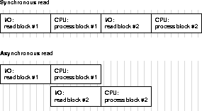
Asynchronous operations are currently supported with parallel table scans and hash joins only. They are not supported for sorts, or for serial table scans. In addition, this feature may require operating system specific configuration and may not be supported on all platforms. Check your Oracle platform-specific documentation.
Note: If asynchronous I/O behavior is not natively available, you can simulate it by deploying I/O server processes using the following parameters: DBWR_IO_SLAVES, LGWR_IO_SLAVES, BACKUP_DISK_IO_SLAVES, and BACKUP_TAPE_IO_SLAVES. Whether or not you use I/O servers is independent of the availability of asynchronous I/O from the platform. Although I/O server processes can be deployed even when asynchronous I/O is available, Oracle does not recommend this practice.
This section describes how to tune the physical database layout for optimal performance of parallel execution.
Different parallel operations use different types of parallelism. The physical database layout you choose should depend on what parallel operations are most prevalent in your application.
The basic unit of parallelism is a called a granule. The operation being parallelized (a table scan, table update, or index creation, for example) is divided by Oracle into granules. Parallel server processes execute the operation one granule at a time. The number of granules and their size affect the degree of parallelism you can use, and how well the work is balanced across parallel server processes.
Block range granules are the basic unit of most parallel operations (exceptions include such operations as parallel DML and CREATE LOCAL INDEX). This is true even on partitioned tables; it is the reason why, on Oracle, the parallel degree is not related to the number of partitions. Block range granules are ranges of physical blocks from the table. Because they are based on physical data addresses, you can size block range granules to allow better load balancing. Block range granules permit dynamic parallelism that does not depend on static preallocation of tables or indexes. On SMP systems granules are located on different devices in order to drive as many disks as possible. On many MPP systems, block range granules are preferentially assigned to parallel server processes that have physical proximity to the disks storing the granules. Block range granules are used with global striping.
When block range granules are used predominantly for parallel access to a table or index, administrative considerations such as recovery, or using partitions for deleting portions of data, may influence partition layout more than performance considerations. If parallel execution operations frequently take advantage of partition pruning, it is important that the set of partitions accessed by the query be striped over at least as many disks as the degree of parallelism.
See Also: For MPP systems, see your platform-specific documentation
When partition granules are used, a parallel server process works on an entire partition of a table or index. Because partition granules are statically determined when a table or index is created, partition granules do not allow as much flexibility in parallelizing an operation. This means that the degree of parallelism possible might be limited, and that load might not be well balanced across parallel server processes.
Partition granules are the basic unit of parallel index range scans and parallel operations that modify multiple partitions of a partitioned table or index. These operations include parallel update, parallel delete, parallel direct-load insert into partitioned tables, parallel creation of partitioned indexes, and parallel creation of partitioned tables.
When partition granules are used for parallel access to a table or index, it is important that there be a relatively large number of partitions (at least three times the degree of parallelism), so that work can be balanced across the parallel server processes.
See Also: Oracle8 Concepts for information on disk striping and partitioning.
To avoid I/O bottlenecks, you should stripe all tablespaces accessed in parallel over at least as many disks as the degree of parallelism. Stripe over at least as many devices as CPUs. You should stripe tablespaces for tables, tablespaces for indexes, and temporary tablespaces. You must also spread the devices over controllers, I/O channels, and/or internal busses.
To stripe data during load, use the FILE= clause of parallel loader to load data from multiple load sessions into different files in the tablespace. For any striping to be effective, you must ensure that enough controllers and other I/O components are available to support the bandwidth of parallel data movement into and out of the striped tablespaces.
The operating system or volume manager can perform striping (OS striping), or you can perform striping manually for parallel operations.
Operating system striping with a large stripe size (at least 64K) is recommended, when possible. This approach always performs better than manual striping, especially in multi-user environments.
Operating system striping is usually flexible and easy to manage. It supports multiple users running sequentially as well as single users running in parallel. Two main advantages make OS striping preferable to manual striping, unless the system is very small or availability is the main concern:
Stripe size must be at least as large as the I/O size. If stripe size is larger than I/O size by a factor of 2 or 4, then certain tradeoffs may arise. The large stripe size can be beneficial because it allows the system to perform more sequential operations on each disk; it decreases the number of seeks on disk. The disadvantage is that it reduces the I/O parallelism so that fewer disks are active at the same time. If you should encounter problems in this regard, increase the I/O size of scan operations (going, for example, from 64K to 128K), rather than changing the stripe size. Note that the maximum I/O size is platform specific (in a range, for example, of 64K to 1MB).
With OS striping, from a performance standpoint, the best layout is to stripe data, indexes, and temporary tablespaces across all the disks of your platform. In this way, maximum I/O performance (both in term of throughput and number of I/Os per second) can be reached when one object is accessed by a parallel operation. If multiple objects are accessed at the same time (as in a multi-user configuration), striping will automatically limit the contention. If availability is a major concern, associate this scheme with hardware redundancy (for example RAID5), which permits both performance and availability.
Manual striping can be done on all platforms. This requires more DBA planning and effort to set up. For manual striping add multiple files, each on a separate disk, to each tablespace. The main problem with manual striping is that the degree of parallelism is more a function of the number of disks than of the number of CPUs. This is because it is necessary to have one server process per datafile to drive all the disks and limit the risk of being I/O bound. Also, this scheme is very sensitive to any skew in the datafile size which can affect the scalability of parallel scan operations.
Local striping, which applies only to partitioned tables and indexes, is a form of non-overlapping disk-to-partition striping. Each partition has its own set of disks and files, as illustrated in Figure 19-6. There is no overlapping disk access, and no overlapping files.
Advantages of local striping are that if one disk fails it will not affect other partitions, and you still have some striping even if you have data in only one partition.
A disadvantage of local striping is that you need many more disks to implement it-each partition requires a few disks of its own. Another major disadvantage is that after partition pruning to only a single or a few partitions, the system will have limited I/O bandwidth. As a result, local striping is not very practical for parallel operations. For this reason, consider local striping only if your main concern is availability, and not parallel execution. A good compromise might be to use global striping associated with RAID5, which permits both performance and availability.
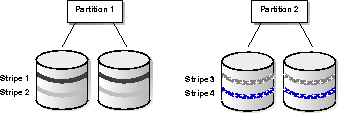 Local Striping
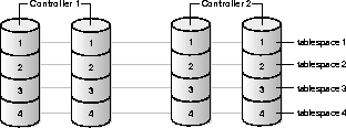
Global striping, illustrated in Figure 19-7, entails overlapping disks and partitions.
 Global Striping
Global striping is advantageous if you have partition pruning and need to access data only in one partition. Spreading the data in that partition across many disks improves performance for parallel query operations. A disadvantage of global striping is that if one disk fails, all partitions are affected.
See Also: "Striping and Media Recovery" on page 19-30
Relationships. To analyze striping, consider the following relationships:
Figure 19-8 shows the cardinality of the relationships between objects in the storage system. For every table there may be p partitions; there may be s partitions for every tablespace, f files for every tablespace, and m files to n devices (a many-to-many relationship).
Goals. You may wish to stripe an object across devices for the sake of one of three goals:
To attain both Goal 1 and Goal 2 (having the table reside on many devices, with the highest possible availability) you can maximize the number of partitions (p) and minimize the number of partitions per tablespace (s).
For highest availability, but least intra-partition parallelism, place each partition in its own tablespace; do not used striped files; and use one file per tablespace. To minimize #2, set f and n equal to 1.
Notice that the solution that minimizes availability maximizes intra-partition parallelism. Goal 3 conflicts with Goal 2 because you cannot simultaneously maximize the formula for Goal 3 and minimize the formula for Goal 2. You must compromise if you are interested in both goals.
Goal 1: To optimize full table scans. Having a table on many devices is beneficial because full table scans are scalable.
Calculate the number of partitions multiplied by the number of files in the tablespace multiplied by the number of devices per file. Divide this product by the number of partitions that share the same tablespace, multiplied by the number of files that share the same device. The formula is as follows:![]()
You can do this by having t partitions, with every partition in its own tablespace, if every tablespace has one file, and these files are not striped.
t x 1/p x 1 x 1, up to t devices
If the table is not partitioned, but is in one tablespace, one file, it should be striped over n devices.
1 x 1 x n
Maximum t partitions, every partition in its own tablespace, f files in each tablespace, each tablespace on striped device:
t x f x n devices
Goal 2: To optimize availability. Restricting each tablespace to a small number of devices and having as many partitions as possible helps you achieve high availability.![]()
Availability is maximized when f = n = m = 1 and p is much greater than 1.
Goal 3: To optimize partition scans. Achieving intra-partition parallelism is beneficial because partition scans are scalable. To do this, place each partition on many devices.![]()
Partitions can reside in a tablespace that can have many files. There could be either
Striping affects media recovery. Loss of a disk usually means loss of access to all objects that were stored on that disk. If all objects are striped over all disks, then loss of any disk takes down the entire database. Furthermore, you may need to restore all database files from backups, even if each file has only a small fraction actually stored on the failed disk.
Often, the same OS subsystem that provides striping also provides mirroring. With the declining price of disks, mirroring can provide an effective supplement to backups and log archival--but not a substitute for them. Mirroring can help your system recover from a device failure more quickly than with a backup, but is not as robust. Mirroring does not protect against software faults and other problems that an independent backup would protect your system against. Mirroring can be used effectively if you are able to reload read-only data from the original source tapes. If you do have a disk failure, restoring the data from the backup could involve lengthy downtime, whereas restoring it from a mirrored disk would enable your system to get back online quickly.
Even cheaper than mirroring is RAID technology, which avoids full duplication in favor of more expensive write operations. For read-mostly applications, this may suffice.
Note: RAID5 technology is particularly slow on write operations. This slowness may affect your database restore time to a point that RAID5 performance is unacceptable.
See Also: For a discussion of manually striping tables across datafiles, refer to "Striping Disks" on page 15-23.
For a discussion of media recovery issues, see "Backup and Recovery of the Data Warehouse" on page 6-8.
For more information about automatic file striping and tools you can use to determine I/O distribution among your devices, refer to your operating system documentation.
Partitioned tables and indexes can improve the performance of operations in a data warehouse. Partitioned tables and indexes allow at least the same parallelism as non-partitioned tables and indexes. In addition, partitions of a table can be pruned based on predicates and values in the partitioning column. Range scans on partitioned indexes can be parallelized, and insert, update and delete operations can be parallelized.
To avoid I/O bottlenecks when not all partitions are being scanned (because some have been eliminated), each partition should be spread over a number of devices. On MPP systems, those devices should be spread over multiple nodes.
Partitioned tables and indexes facilitate administrative operations by allowing them to operate on subsets of data. For example, a new partition can be added, an existing partition can be reorganized, or an old partition can be dropped with less than a second of interruption to a read-only application.
Consider using partitioned tables in a data warehouse when:
If the data being accessed by a parallel operation (after partition pruning is applied) is spread over at least as many disks as the degree of parallelism, then most operations will be CPU-bound and a degree of parallelism ranging from the total number of CPUs to twice that number, is appropriate. Operations that tend to be I/O bandwidth bound can benefit from a higher degree of parallelism, especially if the data is spread over more disks. On sites with multiple users, you might consider using the PARALLEL_ADAPTIVE_MULTI_USER parameter to tune the requested degree of parallelism based on the current number of active parallel execution users. The following discussion is intended more for a single user environment.
Operations that tend to be I/O bandwidth bound are:
Parallel operations that perform random I/O access (such as index maintenance of parallel update and delete operations) can saturate the I/O subsystem with a high number of I/Os, very much like an OLTP system with high concurrency. To ease this I/O problem, the data should be spread among more devices and disk controllers. Increasing the degree of parallelism will not help.
Oracle automatically computes the default parallel degree of a table as the minimum of the number of disks storing the table and the number of CPUs available. If, as recommended, you have striped objects over at least as many disks as you have CPUs, the default parallelism will always be the number of CPUs. Warehouse operations are typically CPU bound; thus the default is a good choice, especially if you are using the asynchronous readahead feature. However, because some operations are by nature synchronous (index probes, for example) an explicit setting of the parallel degree to twice the number of CPUs might be more appropriate. Consider reducing parallelism for objects that are frequently accessed by two or more concurrent parallel operations.
If you find that some operations are I/O bound with the default parallelism, and you have more disks than CPUs, you can override the usual parallelism with a hint that increases parallelism up to the number of disks, or until the CPUs become saturated.
This section presents a case study which illustrates how to create, load, index, and analyze a large data warehouse fact table with partitions, in a typical star schema. This example uses SQL Loader to explicitly stripe data over 30 disks.
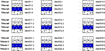 Datafile Layout for Parallel Load Example
Below is the command to create a tablespace named "Tsfacts1". Other tablespaces are created with analogous commands. On a 10-CPU machine, it should be possible to run all 12 CREATE TABLESPACE commands together. Alternatively, it might be better to run them in two batches of 6 (two from each of the three groups of disks).
CREATE TABLESPACE Tsfacts1
DATAFILE /dev/D1.1'  SIZE 1024MB REUSE
DATAFILE /dev/D2.1'  SIZE 1024MB REUSE
DATAFILE /dev/D3.1'  SIZE 1024MB REUSE
DATAFILE /dev/D4.1' SIZE 1024MB REUSE
DATAFILE /dev/D5.1'  SIZE 1024MB REUSE
DATAFILE /dev/D6.1'  SIZE 1024MB REUSE
DATAFILE /dev/D7.1'  SIZE 1024MB REUSE
DATAFILE /dev/D8.1' SIZE 1024MB REUSE
DATAFILE /dev/D9.1'  SIZE 1024MB REUSE
DATAFILE /dev/D10.1  SIZE 1024MB REUSE
DEFAULT STORAGE (INITIAL 100MB NEXT 100MB PCTINCREASE 0)
CREATE TABLESPACE Tsfacts2
DATAFILE /dev/D4.2' SIZE 1024MB REUSE
DATAFILE /dev/D5.2'  SIZE 1024MB REUSE
DATAFILE /dev/D6.2'  SIZE 1024MB REUSE
DATAFILE /dev/D7.2'  SIZE 1024MB REUSE
DATAFILE /dev/D8.2' SIZE 1024MB REUSE
DATAFILE /dev/D9.2'  SIZE 1024MB REUSE
DATAFILE /dev/D10.2  SIZE 1024MB REUSE
DATAFILE /dev/D1.2'  SIZE 1024MB REUSE
DATAFILE /dev/D2.2'  SIZE 1024MB REUSE
DATAFILE /dev/D3.2'  SIZE 1024MB REUSE
DEFAULT STORAGE (INITIAL 100MB NEXT 100MB PCTINCREASE 0)
...
CREATE TABLESPACE Tsfacts4
DATAFILE /dev/D10.4'  SIZE 1024MB REUSE
DATAFILE /dev/D1.4'  SIZE 1024MB REUSE
DATAFILE /dev/D2.4'  SIZE 1024MB REUSE
DATAFILE /dev/D3.4  SIZE 1024MB REUSE
DATAFILE /dev/D4.4' SIZE 1024MB REUSE
DATAFILE /dev/D5.4'  SIZE 1024MB REUSE
DATAFILE /dev/D6.4'  SIZE 1024MB REUSE
DATAFILE /dev/D7.4'  SIZE 1024MB REUSE
DATAFILE /dev/D8.4' SIZE 1024MB REUSE
DATAFILE /dev/D9.4'  SIZE 1024MB REUSE
DEFAULT STORAGE (INITIAL 100MB NEXT 100MB PCTINCREASE 0)
...
CREATE TABLESPACE Tsfacts12
DATAFILE /dev/D30.4'  SIZE 1024MB REUSE
DATAFILE /dev/D21.4'  SIZE 1024MB REUSE
DATAFILE /dev/D22.4'  SIZE 1024MB REUSE
DATAFILE /dev/D23.4  SIZE 1024MB REUSE
DATAFILE /dev/D24.4' SIZE 1024MB REUSE
DATAFILE /dev/D25.4'  SIZE 1024MB REUSE
DATAFILE /dev/D26.4'  SIZE 1024MB REUSE
DATAFILE /dev/D27.4'  SIZE 1024MB REUSE
DATAFILE /dev/D28.4' SIZE 1024MB REUSE
DATAFILE /dev/D29.4'  SIZE 1024MB REUSE
DEFAULT STORAGE (INITIAL 100MB NEXT 100MB PCTINCREASE 0)
Extent sizes in the STORAGE clause should be multiples of the multiblock read size, where
blocksize * MULTIBLOCK_READ_COUNT = multiblock read size
Note that INITIAL and NEXT should normally be set to the same value. In the case of parallel load, make the extent size large enough to keep the number of extents reasonable, and to avoid excessive overhead and serialization due to bottlenecks in the data dictionary. When PARALLEL=TRUE is used for parallel loader, the INITIAL extent is not used. In this case you can override the INITIAL extent size specified in the tablespace default storage clause with the value that you specify in the loader control file (such as, for example, 64K).
Tables or indexes can have an unlimited number of extents provided you have set the COMPATIBLE system parameter and use the MAXEXTENTS keyword on the CREATE or ALTER command for the tablespace or object. In practice, however, a limit of 10,000 extents per object is reasonable. A table or index has an unlimited number of extents, so the PERCENT_INCREASE parameter should be set to zero in order to have extents of equal size.
Note: It is not desirable to allocate extents faster than about 2 or 3 per minute. See "ST (Space Transaction) Enqueue for Sorts and Temporary Data" on page 20-12 for more information. Thus, each process should get an extent that will last for 3 to 5 minutes. Normally such an extent is at least 50MB for a large object. Too small an extent size will incur a lot of overhead, and this will affect performance and scalability of parallel operations. The largest possible extent size for a 4GB disk evenly divided into 4 partitions is 1GB. 100MB extents should work nicely. Each partition will have 100 extents. The default storage parameters can be customized for each object created in the tablespace, if needed.
We create a partitioned table with 12 partitions, each in its own tablespace. The table contains multiple dimensions and multiple measures. The partitioning column is named "dim_2" and is a date. There are other columns as well.
CREATE TABLE fact (dim_1 NUMBER, dim_2 DATE, ...
meas_1 NUMBER, meas_2 NUMBER, ... )
PARALLEL
(PARTITION BY RANGE (dim_2)
PARTITION jan95 VALUES LESS THAN ('02-01-1995') TABLESPACE
TSfacts1
PARTITION feb95 VALUES LESS THAN ('03-01-1995') TABLESPACE
TSfacts2
...
PARTITION dec95 VALUES LESS THAN ('01-01-1996') TABLESPACE
TSfacts12)
;
This section describes four alternative approaches to loading partitions in parallel.
The different approaches to loading help you manage the ramifications of the PARALLEL=TRUE keyword of SQL*Loader, which controls whether or not individual partitions are loaded in parallel. The PARALLEL keyword entails restrictions such as the following:
However, regardless of the setting of this keyword, if you have one loader process per partition, you are still effectively loading into the table in parallel.
Case 1
In this approach, assume 12 input files that are partitioned in the same way as your table. The DBA has 1 input file per partition of the table to be loaded. The DBA starts 12 SQL*Loader sessions in parallel, entering statements like these:
SQLLDR DATA=jan95.dat DIRECT=TRUE CONTROL=jan95.ctl
SQLLDR DATA=feb95.dat DIRECT=TRUE CONTROL=feb95.ctl
. . .
SQLLDR DATA=dec95.dat DIRECT=TRUE CONTROL=dec95.ctl
Note that the keyword PARALLEL=TRUE is not set. A separate control file per partition is necessary because the control file must specify the partition into which the loading should be done. It contains a statement such as:
LOAD INTO fact partition(jan95)
Advantages of this approach are that local indexes are maintained by SQL*Loader. You still get parallel loading, but on a partition level-without the restrictions of the PARALLEL keyword.
A disadvantage is that you must partition the input manually.
Case 2
In another common approach, assume an arbitrary number of input files that are not partitioned in the same way as the table. The DBA can adopt a strategy of performing parallel load for each input file individually. Thus if there are 7 input files, the DBA can start 7 SQL*Loader sessions, using statements like the following:
SQLLDR DATA=file1.dat DIRECT=TRUE PARALLEL=TRUE
Oracle will partition the input data so that it goes into the correct partitions. In this case all the loader sessions can share the same control file, so there is no need to mention it in the statement.
The keyword PARALLEL=TRUE must be used because each of the 7 loader sessions can write into every partition. (In case 1, every loader session would write into only 1 partition, because the data was already partitioned outside Oracle.) Hence all the PARALLEL keyword restrictions are in effect.
In this case Oracle attempts to spread the data evenly across all the files in each of the 12 tablespaces-however an even spread of data is not guaranteed. Moreover, there could be I/O contention during the load when the loader processes are attempting simultaneously to write to the same device.
Case 3
In Case 3 (illustrated in the example), the DBA wants precise control of the load. To achieve this the DBA must partition the input data in the same way as the datafiles are partitioned in Oracle.
This example uses 10 processes loading into 30 disks. To accomplish this, the DBA must split the input into 120 files beforehand. The 10 processes will load the first partition in parallel on the first 10 disks, then the second partition in parallel on the second 10 disks, and so on through the 12th partition. The DBA runs the following commands concurrently as background processes:
SQLLDR DATA=jan95.file1.dat DIRECT=TRUE PARALLEL=TRUE FILE=/dev/D1.1
...
SQLLDR DATA=jan95.file10.dat DIRECT=TRUE PARALLEL=TRUE FILE=/dev/D10.1
WAIT;
...
SQLLDR DATA=dec95.file1.dat DIRECT=TRUE PARALLEL=TRUE FILE=/dev/D30.4
...
SQLLDR DATA=dec95.file10.dat DIRECT=TRUE PARALLEL=TRUE FILE=/dev/D29.4
For Oracle Parallel Server, divide the loader session evenly among the nodes. The datafile being read should always reside on the same node as the loader session. NFS mount of the data file on a remote node is not an optimal approach.
The keyword PARALLEL=TRUE must be used, because multiple loader sessions can write into the same partition. Hence all the restrictions entailed by the PARALLEL keyword are in effect. An advantage of this approach, however, is that it guarantees that all of the data will be precisely balanced, exactly reflecting your partitioning.
Note: Although this example shows parallel load used with partitioned tables, the two features can be used independent of one another.
Case 4
For this approach, all of your partitions must be in the same tablespace. You need to have the same number of input files as datafiles in the tablespace, but you do not need to partition the input the same way in which the table is partitioned.
For example, if all 30 devices were in the same tablespace, then you would arbitrarily partition your input data into 30 files, then start 30 SQL*Loader sessions in parallel. The statement starting up the first session would be like the following:
SQLLDR DATA=file1.dat DIRECT=TRUE PARALLEL=TRUE FILE=/dev/D1
. . .
SQLLDR DATA=file30.dat DIRECT=TRUE PARALLEL=TRUE FILE=/dev/D30
The advantage of this approach is that, as in Case 3, you have control over the exact placement of datafiles, because you use the FILE keyword. However, you are not required to partition the input data by value: Oracle does that.
A disadvantage is that this approach requires all the partitions to be in the same tablespace; this minimizes availability.
For optimal space management performance you can use dedicated temporary tablespaces. As with the TSfacts tablespace, we first add a single datafile and later add the remainder in parallel.
CREATE TABLESPACE TStemp TEMPORARY DATAFILE '/dev/D31'
SIZE 4096MB REUSE
DEFAULT STORAGE (INITIAL 10MB NEXT 10MB PCTINCREASE 0);
Temporary extents are all the same size, because the server ignores the PCTINCREASE and INITIAL settings and only uses the NEXT setting for temporary extents. This helps to avoid fragmentation.
As a general rule, temporary extents should be smaller than permanent extents, because there are more demands for temporary space, and parallel processes or other operations running concurrently must share the temporary tablespace. Normally, temporary extents should be in the range of 1MB to 10MB. Once you allocate an extent it is yours for the duration of your operation. If you allocate a large extent but only need to use a small amount of space, the unused space in the extent is tied up.
At the same time, temporary extents should be large enough that processes do not have to spend all their time waiting for space. Temporary tablespaces use less overhead than permanent tablespaces when allocating and freeing a new extent. However, obtaining a new temporary extent still requires the overhead of acquiring a latch and searching through the SGA structures, as well as SGA space consumption for the sort extent pool. Also, if extents are too small, SMON may take a long time dropping old sort segments when new instances start up.
Operating system striping is an alternative technique you can use with temporary tablespaces. Media recovery, however, offers subtle challenges for large temporary tablespaces. It does not make sense to mirror, use RAID, or back up a temporary tablespace. If you lose a disk in an OS striped temporary space, you will probably have to drop and recreate the tablespace. This could take several hours for our 120 GB example. With Oracle striping, simply remove the bad disk from the tablespace. For example, if /dev/D50 fails, enter:
ALTER DATABASE DATAFILE `/dev/D50' RESIZE 1K;
ALTER DATABASE DATAFILE `/dev/D50' OFFLINE;
Because the dictionary sees the size as 1K, which is less than the extent size, the bad file will never be accessed. Eventually, you may wish to recreate the tablespace.
Be sure to make your temporary tablespace available for use:
ALTER USER scott TEMPORARY TABLESPACE TStemp;
See Also: For MPP systems, see your platform-specific documentation regarding the advisability of disabling disk affinity when using operating system striping.
Indexes on the fact table can be partitioned or non-partitioned. Local partitioned indexes provide the simplest administration. The only disadvantage is that a search of a local non-prefixed index requires searching all index partitions.
The considerations for creating index tablespaces are similar to those for creating other tablespace. Operating system striping with a small stripe width is often a good choice, but to simplify administration it is best to use a separate tablespace for each index. If it is a local index you may want to place it into the same tablespace as the partition to which it corresponds. If each partition is striped over a number of disks, the individual index partitions can be rebuilt in parallel for recovery. Alternatively, operating system mirroring can be used. For these reasons the NOLOGGING option of the index creation statement may be attractive for a data warehouse.
Tablespaces for partitioned indexes should be created in parallel in the same manner as tablespaces for partitioned tables.
Partitioned indexes are created in parallel using partition granules, so the maximum degree of parallelism possible is the number of granules. Local index creation has less inherent parallelism than global index creation, and so may run faster if a higher degree of parallelism is used. The following statement could be used to create a local index on the fact table.
CREATE INDEX I on fact(dim_1,dim_2,dim_3) LOCAL
PARTITION jan95 TABLESPACE Tsidx1,
PARTITION feb95 TABLESPACE Tsidx2,
...
PARALLEL(DEGREE 12) NOLOGGING;
To back up or restore January data, you need only manage tablespace Tsidx1.
See Also: Oracle8 Concepts for a discussion of partitioned indexes.
When parallel insert, update, or delete are to be performed on a data warehouse, some additional considerations are needed when designing the physical database. Note that these considerations do not affect parallel query operations. This section covers:
If you are performing parallel insert, update, or delete operations, the degree of parallelism will be equal to or les than the number of partitions in the table.
See Also: "Determining the Degree of Parallelism" on page 19-32
Parallel DML works mostly on partitioned tables. It does not use asynchronous I/O and may generate a high number of random I/O requests during index maintenance of parallel UPDATE and DELETE operations. For local index maintenance, local striping is most efficient in reducing I/O contention, because one server process will only go to its own set of disks and disk controllers. Local striping also increases availability in the event of one disk failing.
For global index maintenance, (partitioned or non-partitioned), globally striping the index across many disks and disk controllers is the best way to distribute the number of I/Os.
If you have global indexes, a global index segment and global index blocks will be shared by server processes of the same parallel DML statement. Even if the operations are not performed against the same row, the server processes may share the same index blocks. Each server transaction needs one transaction entry in the index block header before it can make changes to a block. Therefore, in the CREATE INDEX or ALTER INDEX statements, you should set INITRANS (the initial number of transactions allocated within each data block) to a large value, such as the maximum degree of parallelism against this index. Leave MAXTRANS, the maximum number of concurrent transactions that can update a data block, at its default value, which is the maximum your system can support (not to exceed 255).
If you run degree 10 parallelism against a table with a global index, all 10 server processes might attempt to change the same global index block. For this reason you must set MAXTRANS to at least 10 so that all the server processes can make the change at the same time. If MAXTRANS is not large enough, the parallel DML operation will fail.
Once a segment has been created, the number of process and transaction free lists is fixed and cannot be altered. If you specify a large number of process free lists in the segment header, you may find that this limits the number of transaction free lists that are available. You can abate this limitation the next time you recreate the segment header by decreasing the number of process free lists; this will leave more room for transaction free lists in the segment header.
For UPDATE and DELETE operations, each server process may require its own transaction free list. The parallel DML degree of parallelism is thus effectively limited by the smallest number of transaction free lists available on any of the global indexes which the DML statement must maintain. For example, if you have two global indexes, one with 50 transaction free lists and one with 30 transaction free lists, the degree of parallelism is limited to 30.
Note that the FREELISTS parameter of the STORAGE clause is used to set the number of process free lists. By default, no process free lists are created.
The default number of transaction free lists depends on the block size. For example, if the number of process free lists is not set explicitly, a 4K block has about 80 transaction free lists by default. The minimum number of transaction free lists is 25.
See Also: Oracle8 Parallel Server Concepts & Administration for information about transaction free lists.
Parallel DDL and parallel DML operations may generate a large amount of redo logs. A single ARCH process to archive these redo logs might not be able to keep up. To avoid this problem, you can spawn multiple archiver processes. This can be done manually or by using a job queue.
Parallel DML operations dirty a large number of data, index, and undo blocks in the buffer cache during a short period of time. If you see a high number of "free_buffer_waits" in the V$SYSSTAT view, tune the DBWn process(es).
See Also: "Tuning the Redo Log Buffer" on page 14-7
The [NO]LOGGING option applies to tables, partitions, tablespaces, and indexes. Virtually no log is generated for certain operations (such as direct-load INSERT) if the NOLOGGING option is used. The NOLOGGING attribute is not specified at the INSERT statement level, but is instead specified when using the ALTER or CREATE command for the table, partition, index, or tablespace.
When a table or index has NOLOGGING set, neither parallel nor serial direct-load INSERT operations generate undo or redo logs. Processes running with the NOLOGGING option set run faster because no redo is generated. However, after a NOLOGGING operation against a table, partition, or index, if a media failure occurs before a backup is taken, then all tables, partitions, and indexes that have been modified may be corrupted.
Note: Direct-load INSERT operations (except for dictionary updates) never generate undo logs. The NOLOGGING attribute does not affect undo, but only redo. To be precise, NOLOGGING allows the direct-load INSERT operation to generate a negligible amount of redo (range-invalidation redo, as opposed to full image redo).
For backward compatibility, [UN]RECOVERABLE is still supported as an alternate keyword with the CREATE TABLE statement in Oracle8 Server, release 8.0. This alternate keyword may not be supported, however, in future releases.
AT the tablespace level, the logging clause specifies the default logging attribute for all tables, indexes, and partitions created in the tablespace. When an existing tablespace logging attribute is changed by the ALTER TABLESPACE statement, then all tables, indexes, and partitions created after the ALTER statement will have the new logging attribute; existing ones will not change their logging attributes. The tablespace level logging attribute can be overridden by the specifications at the table, index, or partition level).
The default logging attribute is LOGGING. However, if you have put the database is in NOARCHIVELOG mode (by issuing ALTER DATABASE NOARCHIVELOG), then all operations that can be done without logging will not generate logs, regardless of the specified logging attribute.
See Also: Oracle8 SQL Reference
After the data is loaded and indexed, analyze it. It is very important to analyze the data after any DDL changes or major DML changes. The ANALYZE command does not execute in parallel against a single table or partition. However, many different partitions of a partitioned table can be analyzed in parallel. Use the stored procedure DBMS_UTILITY.ANALYZE_PART_OBJECT to submit jobs to a job queue in order to analyze a partitioned table in parallel.
ANALYZE must be run twice in the following sequence to gather table and index statistics, and to create histograms. (The second ANALYZE statement creates histograms on columns.)
ANALYZE TABLE xyz ESTIMATE STATISTICS;
ANALYZE TABLE xyz ESTIMATE STATISTICS FOR ALL COLUMNS;
ANALYZE TABLE gathers statistics at the table level (for example, the number of rows and blocks), and for all dependent objects, such as columns and indexes. If run in the reverse sequence, the table-only ANALYZE will destroy the histograms built by the column-only ANALYZE.
An ESTIMATE of statistics produces accurate histograms for small tables only. Once the table is more than a few thousand rows, accurate histograms can only be ensured if more than the default number of rows is sampled. The sample size you choose depends on several factors: the objects to be analyzed (table, indexes, columns); the nature of the data (skewed or not); whether you are building histograms; as well as the performance you expect. The sample size for analyzing an index or a table need not be big; 1 percent is more than enough for tables containing more than 2000 rows.
Queries with many joins are quite sensitive to the accuracy of the statistics. Use the COMPUTE option of the ANALYZE command if possible (it may take quite some time and a large amount of temporary space). If you must use the ESTIMATE option, sample as large a percentage as possible (for example, 10%). If you use too high a sample size for ESTIMATE, however, this process may require practically the same execution time as COMPUTE. A good rule of thumb, in this case, is not to choose a percentage which causes you to access every block in the system. For example, if you have 20 blocks, and each block has 1000 rows, estimating 20% will cause you to touch every block. You may as well have computed the statistics!
Use histograms for data that is not uniformly distributed. Note that a great deal of data falls into this classification.
When you analyze a table, Oracle also analyzes all the different objects that are defined on that table: the table as well as its columns and indexes. Note that you can use the ANALYZE INDEX statement to analyze the index separately. You may wish to do this when you add a new index to the table; it enables you to specify a different sample size. You can analyze all partitions of facts (including indexes) in parallel in one of two ways:
EXECUTE DBMS_UTILITY.ANALYZE_PART_OBJECT(OBJECT_NAME=>'facts',
COMMAND_TYPE=>'C');
It is worthwhile computing or estimating with a larger sample size the indexed columns, rather than the measure data. The measure data is not used as much: most of the predicates and critical optimizer information comes from the dimensions. A DBA should know which columns are the most frequently used in predicates.
For example, you might analyze the data in two passes. In the first pass you could obtain some statistics by analyzing 1% of the data. Run the following command to submit analysis commands to the job queues:
EXECUTE DBMS_UTILITY.ANALYZE_PART_OBJECT(OBJECT_NAME=>'facts',
COMMAND_TYPE=>'E',
SAMPLE_CLAUSE=>'SAMPLE 1 PERCENT');
In a second pass, you could refine statistics for the indexed columns and the index (but not the non-indexed columns):
EXECUTE DBMS_UTILITY.ANALYZE_PART_OBJECT(OBJECT_NAME=>'facts',
COMMAND_TYPE=>'C',
COMMAND_OPT=>'FOR ALL INDEXED
COLUMNS SIZE 1');
EXECUTE DBMS_UTILITY.ANALYZE_PART_OBJECT(OBJECT_NAME=>'facts',
COMMAND_TYPE=>'C',
COMMAND_OPT=>'FOR ALL INDEXES'):
The result will be a faster plan because you have collected accurate statistics on the most sensitive columns. You are spending more resources to get good statistics on high-value columns (indexes and join columns), and getting baseline statistics for the rest of the data.
Note: Cost-based optimization is always used with parallel execution and with partitioned tables. You must therefore analyze partitioned tables or tables used with parallel query.